

Module 4 · Unit 3
Read the unit content below, then use the case studies and key terms to review what you have learned.
By the end of this session, learners should be able to:
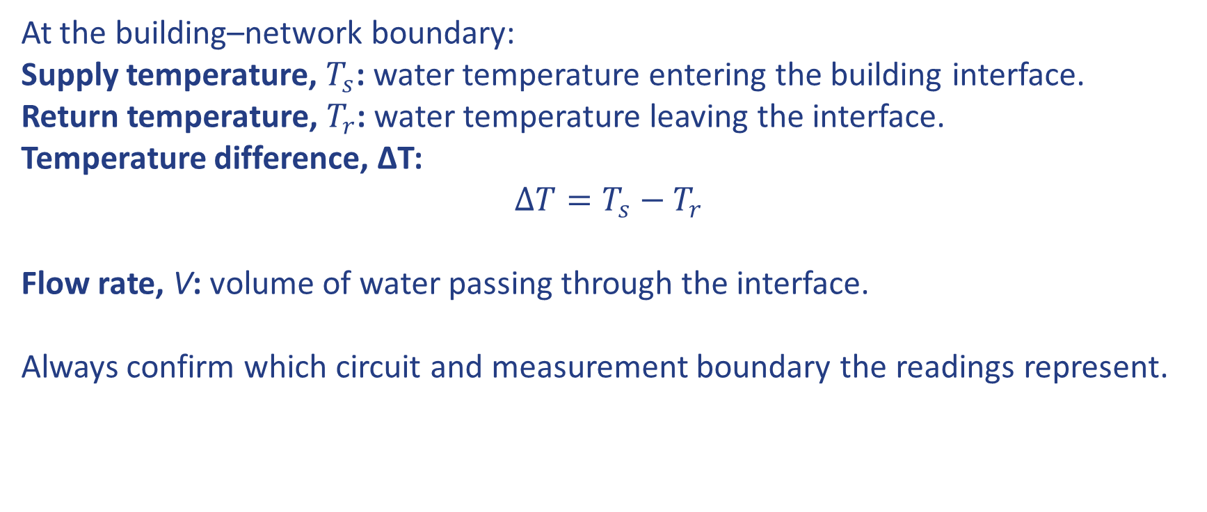
At the building–network boundary:
Supply temperature, : water temperature entering the building interface.
Return temperature, : water temperature leaving the interface.
Temperature difference, ΔT:
Flow rate, V: volume of water passing through the interface.
Always confirm which circuit and measurement boundary the readings represent.
For a fixed heat duty, required flow is inversely proportional to ΔT.
high return temperature → low ΔT → increased flow rate Vm3/h
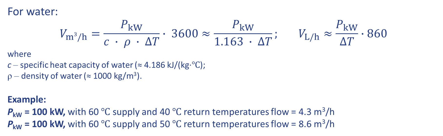
For water:
where
c – specific heat capacity of water (≈ 4.186 kJ/(kg∙℃);
ρ – density of water (≈ 1000 kg/m3).
Example:
PkW = 100 kW, with 60 ℃ supply and 40 ℃ return temperatures flow = 4.3 m3/h
PkW = 100 kW, with 60 ℃ supply and 50 ℃ return temperatures flow = 8.6 m3/h
For the required heat duty, a suitable low return temperature can support:
Operating principle
Deliver the required comfort and DHW service with the lowest practical return temperature and appropriate flow—without compromising hygiene, safety or control stability.
A small ΔT can result from:
Before interpreting ΔT, confirm:
Low Delta T can be a symptom, not a root cause. Interpret it together with power, flow, operating mode and data quality.
Building-side system
Interface controls
Equipment condition
Pumping energy is highly sensitive to flow rates:
In a system dominated by friction losses, doubling flow can approximately quadruple pressure loss and increase hydraulic power by up to roughly eight times (!), depending on pump efficiency and control.
A high return temperature does not itself consume pump energy, but it is often associated with excessive or uncontrolled flow.
Network heat loss is influenced by:
Reducing the average network temperature can:
Lower return temperature helps, but lowering an unnecessarily high supply temperature is often equally or more important.
Condensing boilers
A sufficiently low return temperature supports flue-gas condensation and higher efficiency. Use manufacturer performance data rather than one universal threshold.
Heat pumps
Lower required supply temperature generally reduces temperature lift and improves COP. The effect of network return temperature depends on the plant configuration.
Recovered and renewable heat
Lower network temperatures can make more low-grade heat sources usable.
When poor performance is identified:
Examples of support may include:
1. Verify the data, operating mode and approved design, confirm sensors locations, inspect for leakage, bypass flow and active alarms.
2. Repair failed valves, actuators, sensors, pumps and blocked strainers.
3. Recommission control-valve settings; differential pressure; heating curve; pump mode; DHW and standby settings; hydraulic balancing.
4. Optimise schedules and control logic.
5. Upgrade components where evidence justifies it.
6. Replace or redesign only where existing equipment cannot meet requirements.
7. Verify and document the result.
Compare performance before and after the intervention under similar conditions.
Do not begin with equipment replacement when a sensor, setting or balancing fault may be responsible.
Optimisation starts where heat is actually used.
Hydraulic balancing aims to ensure that each emitter receives the flow needed to meet demand—without excessive circulation.
Possible methods include:
Signs of poor balancing can include:
Check:
A control valve cannot provide stable control if it is oversized or exposed to unsuitable differential pressure.
The control system should:
Weather compensation is a control strategy that automatically adjusts the supply flow temperature based on the outside air temperature.
How it works: As the outdoor temperature rises and the building's heat demand falls, the controller follows a "compensation curve" to lower the flow temperature.
Impact: Lowering the flow temperature during milder weather reduces heat losses from distribution pipework and improves the efficiency of heat sources.
A monitoring system normally includes:
Useful system requirements include:
Core interface data
| Purpose | Indicative interval |
|---|---|
| Billing | monthly or jurisdictional requirement |
| Long-term performance | hourly or half-hourly |
| Daily control behaviour | 5–15 minutes |
| DHW draws or rapid oscillation | shorter interval where technically available |
Step 1 — Validate the data
Check:
Step 2 — Identify the operating mode
Separate:
Step 3 — Compare with the appropriate target
Do not compare every reading with one universal ΔT value. Use a mode- and load-specific return-temperature or ΔT target.
Step 4 — Describe the symptom
Examples:
Step 5 — Choose the first check
Step 6 — Escalate if required
Step 7 — Verify the outcome
Repeat measurements under comparable operating conditions and document the result.
Readings
Primary supply: 80°C
Primary return: 79°C
Flow: continuously high
Dwelling demand: zero
Observation: end-of-lateral bypass pipework is warm
Questions
What is the ΔT?
What does the combination of high flow and 1 K ΔT suggest?
What should be checked first?
Who should authorise any valve adjustment?
Evidence
DHW outlet temperature: 48°C
Project target: 55°C
Complaint occurs between 18:00 and 20:00
Differential pressure at the dwelling connection falls during the same period
Performance is acceptable outside the peak period
Questions
What does the timing suggest?
Which evidence should be checked next?
Is the likely issue local, network-wide or still uncertain?
Who should investigate?
Escalation responsibilities depend on project contracts and the learner’s authorised role.
| Symptom | Safe first check | Typical escalation |
|---|---|---|
| High flow during zero demand | Confirm mode; inspect schematic and bypass status | Maintenance/commissioning |
| High return during heating | Review heating curve, flow and balancing evidence | Commissioning specialist |
| DHW temperature instability | Compare DHW, primary temperature, flow and differential pressure | Controls or network operator |
| Oscillating flow/temperature | Check trend interval, valve signal and pressure variation | BMS/controls specialist |
| Missing or frozen data | Check power, communication and time stamps | Metering/communications provider |
| Repeated blockage or fouling | Inspect strainers and water-quality records | Maintenance/water-treatment specialist |
The temperature of district-network water entering and leaving the substation or consumer connection. It is a boundary condition for heat-exchanger duty and building-side temperatures. A low and stable primary return temperature is generally beneficial because it can reduce required network flow and support efficient heat generation and low-temperature source integration. It does not, by itself, prove that comfort, duty or control requirements are being met.
The flow and return temperatures in the building-side heating circuit downstream of an indirect heat exchanger. The secondary return temperature places a practical lower limit on the achievable primary return temperature, subject to the heat exchanger approach temperature and operating conditions.
The temperature difference between two stated measurement points. At a district-heating interface, primary ΔT is normally calculated as primary supply temperature minus primary return temperature. The circuit, measurement points, operating mode and averaging period must always be stated.
The temperature difference selected for a defined design duty and set of boundary conditions, such as outdoor design temperature, primary supply temperature and secondary heating regime. Separate design values may be required for space heating, DHW production, standby and part-load operation.
The measured temperature difference during real operation. It varies with load, supply temperature, cold-water temperature, emitter control, flow rate and transients, so a single instantaneous value should not be treated as a complete measure of annual performance.
A specified maximum or expected return temperature for a stated operating condition or reporting period. A target may be fixed, weather-dependent, mode-specific or load-dependent; it should be achievable without compromising heat delivery, hygiene, safety or thermal comfort.
For a single-phase water circuit, the transferred heat rate is approximately Q̇ = ṁ × cp × ΔT, where ṁ is mass flow rate and cp is specific heat capacity. The relationship explains why, for the same heat duty and fluid properties, a smaller ΔT requires a larger flow rate.
The quantity of fluid passing a point per unit time, expressed as mass flow or volumetric flow. Flow must be interpreted together with heat duty and ΔT: high flow is not automatically a fault, but flow above that needed for the delivered duty indicates poor use of hydraulic capacity.
Persistent operation with a smaller temperature difference, or greater specific volume flow, than intended for the delivered heat. It is commonly associated with elevated return temperature and excess flow, but diagnosis must also consider supply temperature, load, sensor accuracy and whether the design target is applicable to the observed mode.
Primary flow greater than that required to meet the actual heat duty at the intended temperature difference. It may result from oversized or poorly controlled valves, excessive differential pressure, constant-flow operation, bypasses or incorrect flow limits, and it consumes network and pumping capacity.
Changes in the pressure difference available across the consumer connection as pumps and other customers modulate. Without suitable pressure control, these variations change valve flow for the same opening position and can cause overflow, noise, hunting or insufficient duty.
Control-valve sizing determines the flow coefficient available at the design duty. Valve authority expresses the valve pressure drop relative to the pressure drop of the controlled circuit. An oversized valve or low authority can produce coarse, pressure-sensitive modulation and excess flow; the heat exchanger itself being oversized is not normally a root cause of high return temperature.
Repeated opening and closing or unstable modulation around a setpoint. Hunting can be caused by excessive controller gain, poor sensor response, valve stiction, low valve authority, unsuitable actuator speed, delays or excessive differential pressure, and can produce alternating flow and return-temperature peaks.
Flow that moves from supply to return without delivering the intended useful heat, for example through an open bypass, incorrectly arranged three-way valve, leaking connection or uncontrolled keep-warm path. The effect is usually high return temperature, low ΔT and wasted pumping capacity.
Building-side flow greater than required for the emitted heat. It raises secondary return temperature and, in an indirect connection, usually raises the lowest achievable primary return temperature. Causes include excessive pump head, open balancing valves, inappropriate bypasses and poorly preset emitters.
The ability of radiators, convectors or underfloor systems to deliver the required heat at stated flow, return and room temperatures. Larger or appropriately oversized emitters generally enable lower operating temperatures; high return temperature is more commonly linked to excessive flow, poor balancing, unsuitable controls or insufficient emitter capacity that forces high temperature operation.
A secondary supply-temperature curve or setpoint that is higher than needed can increase secondary and primary return temperatures. A setpoint that is too low can cause valves to remain fully open, high flow and failure to meet comfort, so optimisation must be based on both indoor conditions and interface performance.
DHW recirculation and HIU keep-warm functions maintain readiness but can create continuous low-load primary flow and elevated standby return temperature. Their impact depends on pipe losses, control logic, setpoints, valve leakage and whether heat is transferred usefully during standby.
Bias, poor immersion, slow response, unmatched sensors, incorrect wiring or unsuitable locations can distort calculated ΔT and control decisions. Sensors should measure representative, well-mixed fluid temperatures and be checked against the required accuracy and response time.
A control strategy that resets the secondary supply-temperature setpoint according to outdoor temperature. Correct tuning reduces unnecessarily high temperatures at mild conditions and can lower return temperature, but it must be coordinated with emitter sizing, flow control, occupancy and comfort.
Modulation of flow in response to actual heat demand rather than maintaining constant design flow. It supports low specific volume flow at part load, provided valves, sensors and pumps have sufficient range and stability.
Differential-pressure controllers and pressure-independent control valves stabilise the pressure available to control valves or combine pressure regulation with flow control. They improve repeatability and valve authority but do not independently guarantee low return temperature; setpoints and maximum flows still require commissioning.
A physical or software limit on primary flow. It protects network capacity and can discourage overflow, but it must be high enough to meet verified peak duty and should not be used as a substitute for correct valve sizing, balancing or temperature control.
A valve or control function that reduces flow when measured return temperature exceeds a set limit. It can improve cooling of network water, but aggressive or poorly selected limits can reduce heat delivery, cause comfort problems or interact badly with other controls.
Selection and control of pumps so that delivered head and flow follow the actual system requirement. Excess head can drive overflow and noise, while insufficient head can starve circuits; variable-speed control should therefore use an appropriate differential-pressure reference and minimum operating limits.
Adjustment of branch, lockshield, balancing or pressure-independent radiator valves so each emitter receives the design or required flow. Good balancing prevents nearby circuits from over-flowing and helps the building-side return temperature approach its design value.
Control logic that temporarily gives DHW production precedence over space heating and manages the transition between operating modes. Priority can preserve DHW service, but valve sequencing, pump response and post-draw behaviour must be tuned to avoid excessive primary flow or warm standby returns.
An operating approach that uses only the flow needed to meet load while maintaining the required temperatures and comfort. It is not a fixed minimum-flow rule: the optimum flow changes with load, emitter characteristics and supply temperature.
The process of measuring, adjusting and verifying flow limits, differential pressure, heating curves, valve behaviour, pump settings and return temperatures. Because many faults appear only at part load, cold weather, DHW peaks or standby, optimisation should include seasonal follow-up rather than a single design-point test.
Collection and review of temperatures, flow, heat, differential pressure, valve position, pump status and operating mode over time. Monitoring should use sufficient time resolution to capture DHW draws, control transients and standby behaviour, while retaining aggregated data for long-term trends.
An instantaneous value describes one time point; a time-weighted average gives equal importance to each period; a volume-weighted average gives greater importance to periods with greater water flow. The selected method must match the performance question, because the same installation can appear different under each metric.
A return-temperature metric calculated separately for space heating, DHW, keep-warm, standby or other operating modes. Mode separation helps identify the source of poor annual performance and avoids masking a serious standby or DHW fault within a favourable heating-season average.
A metric describing how often and by how much return temperature exceeds a defined target. Percentage of time or volume above target identifies persistence, while temperature-degree-hours or volume-weighted exceedance can reflect severity.
Assessment of sensor accuracy, flow-meter range, timing alignment, missing data, outliers and operating-mode classification before KPIs are interpreted. ΔT becomes especially uncertain when the difference between two temperatures is small or when the sensors are not a matched pair.
Comparison of an interface against its design target, its own historical baseline, comparable connections or network thresholds. Fair benchmarking should account for supply temperature, outdoor conditions, load, DHW cold-water temperature, occupancy and interface type rather than relying only on an unadjusted network average.
For a given heat demand, low ΔT increases required flow and therefore uses more pipe and pump capacity. Aggregate excess flow can increase pumping electricity, differential-pressure problems and hydraulic bottlenecks and may restrict additional connections even when sufficient heat-generation capacity exists.
Lower return temperatures can improve the usable output or efficiency of condensing boilers, heat pumps, CHP heat recovery, flue-gas condensation, solar thermal, geothermal and low-grade excess-heat sources, depending on plant configuration. The benefit is source-specific and should be evaluated using actual plant performance curves.
Return temperature contributes to the mean network temperature and therefore to heat exchange with the surroundings. Lower return temperature generally reduces distribution loss, but the total effect also depends on supply temperature, pipe insulation, ground temperature, flow, network length and operating hours.
A tariff component that rewards low return temperature or low specific volume flow, or charges for performance above a threshold. It can align customer and network incentives, but thresholds, weather adjustment, metering quality and responsibilities for building-side faults must be transparent.
The practice-question document includes answers and explanations for self-study.
When you are ready, take the Unit 3 quiz.